This feels pretty fucking dumb.
- 0 Posts
- 21 Comments
Joined 1 year ago
Cake day: June 14th, 2023
You are not logged in. If you use a Fediverse account that is able to follow users, you can follow this user.
Ain’t nothin’ but a heartache.
The punchline here is a little compact. I don’t feel like it really gives the closure I need. Maybe if the basis for the joke had more continuity the humor would be less discrete.
...
Just kidding.
Operating System Concepts by Silberschatz, Galvin and Gagne is a classic OS textbook. Andrew Tanenbaum has some OS books too. I really liked his OS Design and Implementation book but I’m pretty sure that one is super outdated by now. I have not read his newer one but it is called Modern Operating Systems iirc.

i has nice real world analogues in the form of rotations by pi/2 about the origin (though this depends a little bit on what you mean by “real world analogue”).
Since i=exp(ipi/2), if you take any complex number z and write it in polar form z=rexp(it), then multiplication by i yields a rotation of z by pi/2 about the origin because zi=rexp(it)exp(ipi/2)=rexp(i(t+pi/2)) by using rules of exponents for complex numbers.
More generally since any pair of complex numbers z, w can be written in polar form z=rexp(it), w=uexp(iv) we have wz=(ru)exp(i(t+v)). This shows multiplication of a complex number z by any other complex number w can be thought of in terms of rotating z by the angle that w makes with the x axis (i.e. the angle v) and then scaling the resulting number by the magnitude of w (i.e. the number u)
Alternatively you can get similar conclusions by Demoivre’s theorem if you do not like complex exponentials.
They don’t eventually become 1. Their limit is 1 but none of the terms themselves are 1.
A sequence, its terms and its limit (if it has one) are all different things. The notation 0.999… represents a limit of a particular sequence, not the sequence itself nor the individual terms of the sequence.
For example the sequence 1, 1/2, 1/3, 1/4, … has terms that get closer and closer to 0, but no term of this sequence is 0 itself.
Look at this graph. If you graph the sequence I just mentioned above and connect each dot you will get the graph shown in this picture (ignoring the portion to the left of x=1).
As you go further and further out along this graph in the positive x direction, the curve that is shown gets closer and closer to the x-axis (where y=0). In a sense the curve is approaching the value y=0. For this curve we could certainly use wordings like “the value the curve approaches” and it would be pretty clear to me and you that we don’t mean the values of the curve itself. This is the kind of intuition that we are trying to formalize when we talk about limits (though this example is with a curve rather than a sequence).
Our sequence 0.9, 0.99, 0.999, … is increasing towards 1 in a similar manner. The notation 0.999… represents the (limit) value this sequence is increasing towards rather than the individual terms of the sequence essentially.
I have been trying to dodge the actual formal definition of the limit of a sequence this whole time since it’s sort of technical. If you want you can check it out here though (note that implicitly in this link the sequence terms and limit values should all be real numbers).
My degree is in mathematics. This is not how these notations are usually defined rigorously.
The most common way to do it starts from sequences of real numbers, then limits of sequences, then sequences of partial sums, then finally these notations turn out to just represent a special kind of limit of a sequence of partial sums.
If you want a bunch of details on this read further:
A sequence of real numbers can be thought of as an ordered nonterminating list of real numbers. For example: 1, 2, 3, … or 1/2, 1/3, 1/4, … or pi, 2, sqrt(2), 1000, 543212345, … or -1, 1, -1, 1, … Formally a sequence of real numbers is a function from the natural numbers to the real numbers.
A sequence of partial sums is just a sequence whose terms are defined via finite sums. For example: 1, 1+2, 1+2+3, … or 1/2, 1/2 + 1/4, 1/2 + 1/4 + 1/8, … or 1, 1 + 1/2, 1 + 1/2 + 1/3, … (do you see the pattern for each of these?)
The notion of a limit is sort of technical and can be found rigorously in any calculus book (such as Stewart’s Calculus) or any real analysis book (such as Rudin’s Principles of Mathematical Analysis) or many places online (such as Paul’s Online Math Notes). The main idea though is that sometimes sequences approximate certain values arbitrarily well. For example the sequence 1, 1/2, 1/3, 1/4, … gets as close to 0 as you like. Notice that no term of this sequence is actually 0. As another example notice the terms of the sequence 9/10, 9/10 + 9/100, 9/10 + 9/100 + 9/1000, … approximate the value 1 (try it on a calculator).
I want to stop here to make an important distinction. None of the above sequences are real numbers themselves because lists of numbers (or more formally functions from N to R) are not the same thing as individual real numbers.
Continuing with the discussion of sequences approximating numbers, when a sequence, call it A, approximates some number L, we say “A converges”. If we want to also specify the particular number that A converges to we say “A converges to L”. We give the number L a special name called “the limit of the sequence A”.
Notice in particular L is just some special real number. L may or may not be a term of A. We have several examples of sequences above with limits that are not themselves terms of the sequence. The sequence 0, 0, 0, … has as its limit the number 0 and every term of this sequence is also 0. The sequence 0, 1, 0, 0, … where only the second term is 1, has limit 0 and some but not all of its terms are 0.
Suppose we define a sequence a1, a2, a3, … where each of the an numbers is one of the numbers from 0, 1, 2, 3, 4, 5, 6, 7, 8 or 9. It can be shown that any sequence of the form a1/10, a1/10 + a2/100, a1/10 + a2/100 + a3/1000, … converges (it is too technical for me to show this here but this is explained briefly in Rudin ch 1 or Hrbacek/Jech’s Introduction To Set Theory).
As an example if each of the an values is 1 our sequence of partial sums above simplifies to 0.1,0.11,0.111,… if the an sequence is 0, 2, 0, 2, … our sequence of partial sums is 0.0, 0.02, 0.020, 0.0202, …
We define the notation 0 . a1 a2 a3 … to be the limit of the sequence of partial sums a1/10, a1/10 + a2/100, a1/10 + a2/100 + a3/1000, … where the an values are all chosen as mentioned above. This limit always exists as specified above also.
In particular 0 . a1 a2 a3 … is just some number and it may or may not be distinct from any term in the sequence of sums we used to define it.
When each of the an values is the same number it is possible to compute this sum explicitly. See here (where a=an, r=1/10 and subtract 1 if necessary to account for the given series having 1 as its first term).
So by definition the particular case where each an is 9 gives us our definition for 0.999…
To recap: the value of 0.999… is essentially just whatever value the (simplified) sequence of partial sums 0.9, 0.99, 0.999, … converges to. This is not necessarily the value of any one particular term of the sequence. It is the value (informally) that the sequence is approximating. The value that the sequence 0.9, 0.99, 0.999, … is approximating can be proved to be 1. So 0.999… = 1, essentially by definition.
Some software can be pretty resilient. I ended up watching this video here recently about running doom using different values for the constant pi that was pretty nifty.
What exactly do you think notations like 0.999… and 0.333… mean?
Yes, informally in the sense that the error between the two numbers is “arbitrarily small”. Sometimes in introductory real analysis courses you see an exercise like: “prove if x, y are real numbers such that x=y, then for any real epsilon > 0 we have |x - y| < epsilon.” Which is a more rigorous way to say roughly the same thing. Going back to informality, if you give any required degree of accuracy (epsilon), then the error between x and y (which are the same number), is less than your required degree of accuracy
You are just wrong.
The rigorous explanation for why 0.999…=1 is that 0.999… represents a geometric series of the form 9/10+9/10^2+… by definition, i.e. this is what that notation literally means. The sum of this series follows by taking the limit of the corresponding partial sums of this series (see here) which happens to evaluate to 1 in the particular case of 0.999… this step is by definition of a convergent infinite series.
He is right. 1 approximates 1 to any accuracy you like.

 3·3 months ago
Given that music boxes are very very old it is plausible that beethoven could have made a remark sharing his opinion on this exact issue. I don’t mean to agree/disagree with your point, I just find that kind of interesting.
You’re getting downvoted but you are right. Stuff like this is a super cool example of exactly the type of thing you are talking about imo.
There’s a lot of AI generated art that sucks. But that does not imply that in skilled hands an artist can’t use those tools in creative/interesting ways.
Arguably a lot of these tools are designed specifically to reduce the effort a human has to put in to create the art they want to make too.
Eigenvectors, values, spaces etc are all pretty simple as basic definitions. They just turn out to be essential for the proofs of a lot of nice results in my opinion. Stuff like matrix diagonalization, gram schmidt orthogonalization, polar decomposition, singular value decomposition, pseudoinverses, the spectral theorem, jordan canonical form, rational canonical form, sylvesters law of inertia, a bunch of nice facts about orthogonal and normal operators, some nifty eigenvalue based formulas for the determinant and trace etc.
My experience with eigenstuff has been kind of a slow burn. At first it feels like “that’s it?”, then you do a bunch of tedious calculations that just kind of suck to do… But as you keep going they keep popping up in ways that lead to some really nice results in my opinion.
Oh okay.
If there are infinite numbers, then there’s 3 in there somewhere.
No, this is not true. Just because you have infinitely many numbers in some collection, doesn’t mean one of the numbers in your collection has to be 3.
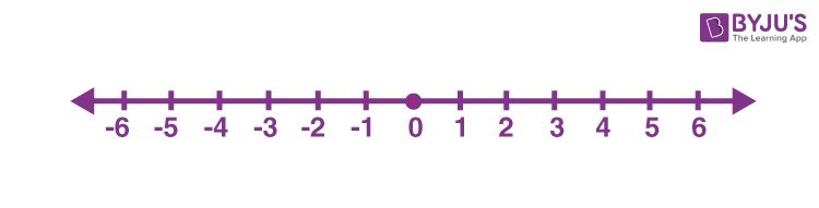
Look at the number line. There are infinitely many numbers on the number line between 1 and 2. For example 1+1/2, 1+1/4, 1+1/8, … are in there (among many others). But all of the numbers between 1 and 2 are strictly smaller than 3, so none of them can be 3.
Alternatively, there are infinitely many numbers strictly smaller than 3, none of which are 3 either.
If 3 is not there then it’s not infinite.
Well consider the set of numbers 3+1, 3+2, 3+3, 3+4, … (the set of integer numbers strictly larger than 3). This set of numbers is also infinite and does not contain 3. So a set being infinite doesn’t imply it must contain the number 3.
I’m sorry my mom called you “pretty fucking dumb”. I know that must have hurt your feelings.